1. Introduction

1.1 Participatory urban planning by smartphone

The smartphone is, nowadays, considered one the most lightweight and common medium to communicate with people. It is believed that the emerging trend “participatory urban planning” can be much facilitated by such technology (Zambonelli et al., 2011); in fact, the mobile phone can capture meaningful information for the participatory planning process. Especially, the mining strategy is to measure the environmental effects of trips by estimating their social costs (Tseng and Hung, 2014).

The smartphone sensors could effectively collect urban trip information using the embedded sensors such as location and accelerometer. Previously, a research (Shin, 2017) presents that the mobile sensing data can be transformed to urban behavior information, especially type of transportation mode information.

1.2 Aims of social cost measurement

In this paper, social costs measurement has a meaning quantify the outcomes of travel and deliver knowledge of its external effects (i.e. the expenses incurred by congestion, noise, accidents, and air, water, and soil pollution, (Camagni et al. 2002)). It was expected that this method, eventually, would also yield an answer to the fundamental question, “How can the data collected from mobile phones contribute useful insight to urban planning?”

In addition, knowing the social costs of travel can deliver precise knowledge on the benefits or side effects of personal choices of travel mode, and may prove the outcome of the planning decision. This is a very important process in urban planning, since it enables visualization of the environmental effects of different travel behaviors. Thus, it can enhance knowledge of the extents to which planning decisions influence the environment, and of which decisions are more profitable in the planning task.

1.3 Social costs estimation of transportation

The urban sensing platform by smartphone presented in this research was intended for operation on the city scale and for management of large datasets.

Social costs estimation in this study was performed according to the following three factors: travel distance, travel mode, and time. Each vehicle type has different cost variables on costs generation; for example, passenger car travel incurs higher social costs than other public transportation, since it has a much higher accidents ratio and produces more environmental pollutions perperson on average. This research utilized the attributes from the report researched by CE Delft and the results that were compiled by other reliable sources (details in Chapter2.2). The referenced reports considered, for the transportation discipline, the following social cost attributes: Congestion, Noise, Accidents, Air pollution, Climate change, Nature & Landscape, and Soil & water pollution.

Social cost estimation will give a sense of environmental effects of personal daily trips by costs. And further, the accumulated total costs will deliver the insight of the environmental influence by transportation policy.

1.4 Research purpose

The primary objective of this study is to analyze the social costs associated with urban planning through the utilization of crowd-sourced mobile sensing data. This research aims to transform complex urban mobility data into actionable insights, thereby facilitating more sustainable and efficient urban planning. By quantifying and evaluating the social costs incurred from various modes of transportation, the study seeks to provide a comprehensive understanding of the impact of urban travel behavior on the broader social and environmental context.

2. Method 1: social costs estimation

2.1 Target social costs typology

With respect to the transportation domain, private costs can be simply measured by their actual expense: for example, personal travel charge, road construction expense, and road facilities management expense. However, in general, external costs are not measurable by such a conventional method. Figure 1 shows a typology of the external cost of transport (Verhoef, 1994). It indicates that road traffic incurs a wide range of social costs, for example, road congestion, noise, accidents, and air, water, and soil pollution. These aspects actually are not visible, and so the relationship between causes and effects is not easy to determine.

Figure 1.

Typology of external costs of transport (Verhoef, 1994)

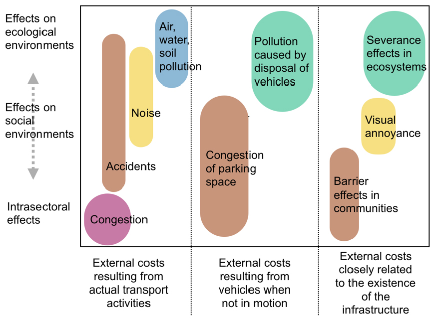
Nevertheless, for the purposes of a sustainable urban environment, such effects cannot be ignored. This is one of the critical criteria for understanding the external effects of current urban transportation. For example, estimating congestion costs and accidents costs will inform on the extent to which citizens’ convenience and safety is secured, and evaluating air, water, and soil pollution by travel can provide an understanding of the likely side effects of travel.

Thereare a number of slightly varying definitions of social cost. Some economists include private cost insocial cost, treating social cost as the total cost to society (Turvey, 1963). In this case, social cost includes both private costs and external costs (Mayeres et al., 1996). Generally speaking though, social costs can be distinguished from private costs so as to indicate only external costs (Walters, 1961). In this study, the latter definition of social costs, which does not include private costs but only external costs as “pure” social costs, was assumed.

2.2 Social costs estimation

As already emphasized, social costs estimation of travel canvary, since the boundary of social costs can be defined based on several different attributes. Therefore, this research first defined the attributes of social costs estimation. The definitions provided by CE Delft, as compiled from several sources (iNFRas, ISI (Institut System-und Innovations forschung), and IMPACT (Internalization Measures and Policies for All external Cost of Transport)) were adopted. The counts costs, then, were derived for the following transportation domainattributes: Congestion, Noise, Accidents, Air pollution, Climate change, Nature & Landscape, and Soil & Water pollution. The other, external aspects, cultural or social behaviors for instance, were not considered in the estimation. The following represent the boundaries of social costs in the transportation sector:

- The social costs estimation of transport in this research used a fixed constant value, which was obtained from the following report: (Maibach et al., 2008), Handbook on estimation of external costs in the transport sector, CE Delft Solutions for environment, economy and technology (www.ce.nl).

- This research first defined the boundary, adopting the definitions provided by CE Delft, and compiled the results by the sources (Figure 2): iNFRas,ISI (Institut System- und Innovations forschung), and IMPACT (Internalization Measures and Policies for All external Cost of Transport).

- The scope of the social costs estimation in this research was transportation. Costs were counted according to the following attributes of the transportation domain: Congestion, Noise, Accidents, Air pollution, Climate change, Nature & Landscape, and Soil & Water pollution.

- Other, external aspects, such as cultural or social behaviors, were not considered in the estimation.

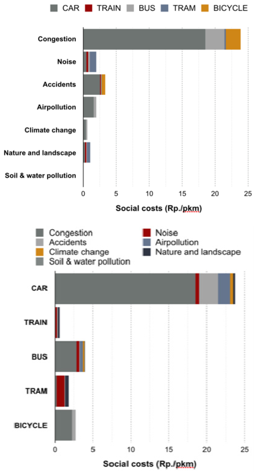
Figure 2.

Incurred social costs of each attribute and each vehicle type (CHF). The graph is a representation of the research outcomes, handbook on estimation of external costs in the transport sector (Maibach et al., 2008)

2.3 Visualization and findings of social costs estimation

The analyzed sensing data was in the form basically of two datasets: travel-mode data, and route information. The route information was simply converted to travel distances. The two datasets were used to measure social costs. The equation is as follows:

Social costs (CHF) = Travel distance (km) × Modes of travel (car, train, bus, tram, bicycle)

A Java-based application was developed to perform the conversion of trips to costs and their visualization. The interface of the application consists of the following four panes (Figure 3): a range slider to select the target group, a Zurich map for individual route visualization, travel information by different vehicle types, and, finally, the calculated social costs of the selection.

First, the planner or the user of the application selects the target group for the measurement (Figure 3, P1), and the target group’s travel will be visualized on the map pane (Figure 3, P2). The user can adjust the target groupby dragging the range sliderbar. Then, the third pane (Figure 3, P3) shows the measured travel information (distance) for each of the travel modes. The fourth pane (Figure 3, P4) shows the final output, which is the amount of the social cost incurred by the trips.

Figure 3.

Visualization of social costs estimation

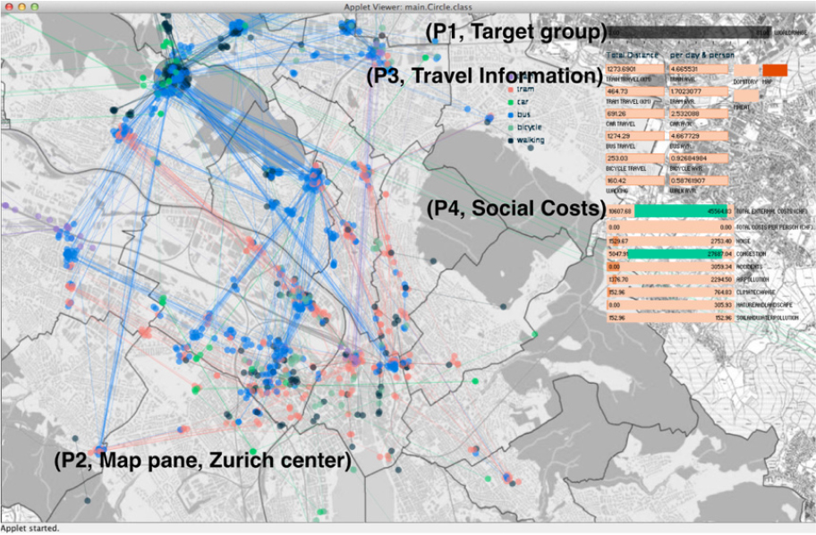
The identified vehicle type and travel distance were used for social costs estimation. The left panel shows the travel routes and identified vehicle types accordingly, and the right panel shows the basic information on the trips as well as the estimated social costs of selected trips.

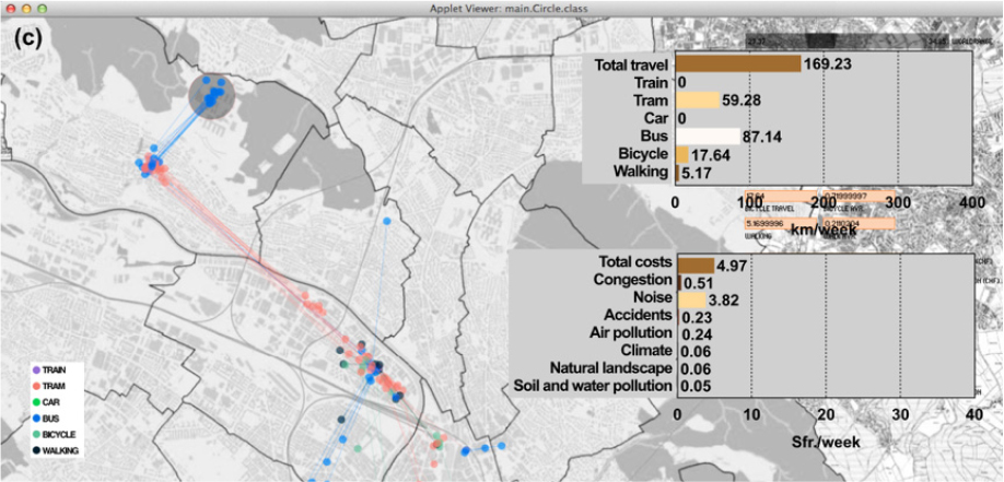
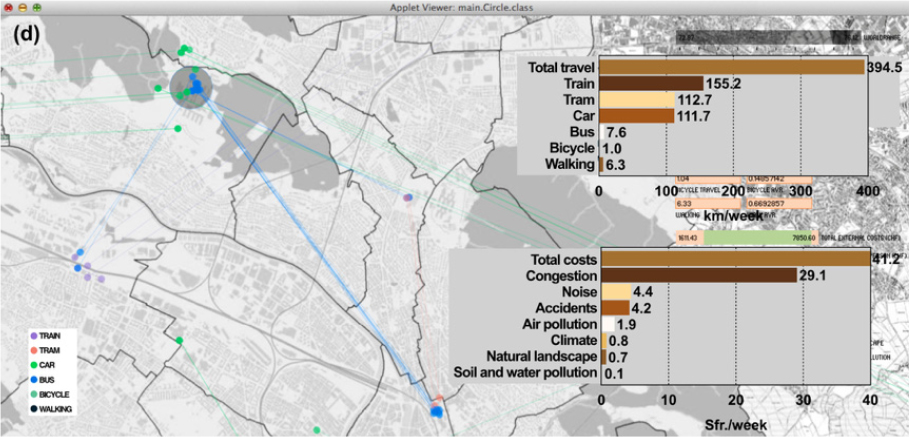
Figure 4 to 7 shows the four different student trip patterns and their social costs analysis:

1) A short-range trip pattern (Figure 4),

2) Two mid-range trip patterns (Figure 5, Figure 6), and

3) A wide-range trip pattern (Figure 7).

Figure 4.

Social cost differences by different trip patterns (Short-range / walking dominant)

Figure 5.

Social cost differences by different trip patterns (Mid-range / tram dominant)

Figure 6.

Social cost differences by different trip patterns (Mid-range / bus dominant)

Figure 7.

Social cost differences by different trip patterns (Wide-range / car dominant)

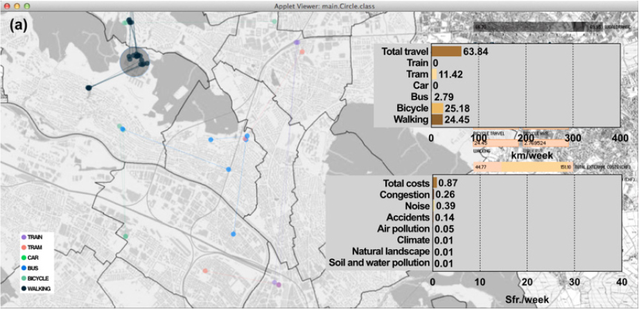
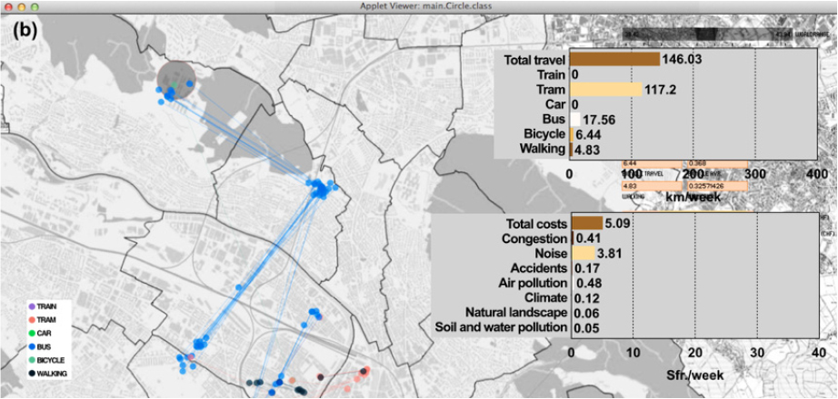
Each travel pattern represents one person’s travel for a week. Each person’s pattern has a different time span in the data. Therefore, it is converted to a week’s average pattern on the basis of a number of trips randomly selected for that week.

The analysis revealed several interesting findings. First, the social costs differ significantly depending on the travel modes. A short-range trip pattern shows a very low level of social costs (CHF 0.87 per week). But obviously, a wide- range travel pattern has significantly higher social costs (CHF 41.20 per week). The wide-range travel pattern plotted in Figure 7 has an only 6-times longer travel distance than the short-range one, and also has same frequency of trips to ETH Hönggerberg, and yet the incurred costs are more than 50 times those of the short-range of travel pattern. This result shows clearly that the different modes of travel exert high leverage effects on social costs.

Another interesting finding is that the mid-range trip pattern (110 km – 170 km per week) accounts for more than 75% of the travels (56 students), and mostly in the mixed- use travel mode. Most mid-range trips tend to consist of diverse travel modes, such as bicycle, bus, tram, and train. Thus, the social costs also tend to converge to the mid-range, or around CHF 4.20 – CHF 6.20.

This finding serves to inform that most people following the mid-range travel pattern (over 75%) generate similar levels of social costs. This is due mostly to the mixed use of travel modes.

3. Method

3.1 Social costs changes by student housing construction

The goal of this chapter is relization of the potentiality of the social costs analysis. First, it was assumed that the social costs analysis could be utilized to determine the building scale and construction site where the most benefit to society could be obtained from the social costs point of view. The aim was to reveal the relationships between different set ups of student housing and transform of travel by analyzing real trip information. The transform of student travel was then evaluated according to the social costs benefits.

The key elements for this analysis are three: 1) existing data: route information of student travel collected by mobile sensing, 2) scenarios: several alternatives for student housing construction (building scale and locations), and 3) costs Analysis: transforms of student travel and the social costs benefits. The analysis steps are as follows:

Step1: find students travel routes and patterns

Step2: evaluate (convert) the trips to social costs.

Step3: show transforms of stocks and flows of student’s trip by different student housing configurations (location and capacity), and define the benefits of the social costs.

3.2 Premises for the experiment

As communicated in the previous chapter, the analyzed sensing data were used for social costs estimation, and the social costs estimation could represent the environmental effects of urban trips. It was assumed that different set ups of student housing would conform to different patterns of students’ trips, and that the changes dependent on the different scenarios will bring different outputs in terms of social costs. The detailed premises areas follows:

a. Social cost values are defined according to the following aspects

- Social costs estimation of transport, as previously, adopts the output of the handbook on estimation of external costs in the transport sector, CE Delft solutions for environment, economy and technology (www.ce.nl).

- Social costs estimation in this research has a limited scope within transportation. It counts costs, as derived from the following attributes of the transportation domain: Congestion, Noise, Accidents, Air pollution, Climate change, Nature & Landscape, and Soil & Water pollution.

b. The travel-pattern data (travel time and date, orientation, destination, vehicle type, distance, frequency) and student housing location & capacity have the following effects:

- The actual travel information is provided by the previous case study of this research.

- The social cost measurement is based on the idea that “stocks and flows (Rotmans et al., 2000) of people travel.” Further details are explained in Chapter 3.3

- Student housing basically reduces existing traffic volume (flow-in) based on its capacity, and increases traffic to the campus and other places (flow-out).

- The deduced traffic (stock = flow in – flow out) will be defined as the final effects of the student housing.

- The student housings reduce (flow-in) travel according to the distance weighting for all of the travel places, such as start, end, and transfer. At the same time, it also increases travels (flow-out) by trips to campus and trips to other places in proportion to the previous travels of the student housing location.

- The stock and flow of travels will be converted to social costs accordingly.

Figure 8 shows the data conversion steps in which the sensing data is converted to social costs suitable for the analysis. Not all of the trip datasets from the all of the students could be collected by crowdsourcing methods. Therefore, the overall collected data should first be converted to real numbers of student trip, after which the converted trips can represent the trips from all students. After that, every trip will be converted to the social costs.

This analysis begins as noted previously: the social costs are mapped on every trip, and are then used to represent all the trips of students.

Figure 8.

Exemplary diagram of social costs analysis process

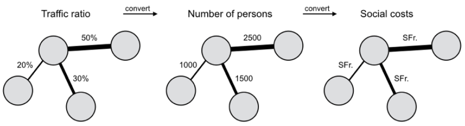
The sensing data informs on which routes are used frequently and which are used less often (Figure 8, left). The traffic ratio data on each route can be obtained by sensing data directly. The traffic ratio is converted into the real number of trips by th etotal numberof students (middle). Finally, each of the trips is converted into a social cost for student housing analysis.

3.3 Definition of social cost stocks and flows

The social cost flow-in, flow-out, and stock are defined (Bontis et al., 2002) as follows:

Definition 1 social cost flow-in: The accommodation scale of each student housing is open parameter, by which the user of the application can set the number prior to the analysis.

One student generates many travels. Thus, the number of accommodated students should be converted into actual numbersof travels. In this calculation, the total number of students’ trips for the student housing is inferred by:

á: the number of trips of á = â: the number of trips of â,

where á is the total number of students, and â is a number of student-housing students.

The reduction ratio by student housing (flow-in) is defined by the distance from it. In order to define the weighting Wj, the calculation takes the following steps:

Arrange all of the travels f(x)i by distance as:

f(x)i=d1+d2+d3+⋯d1×a

All of the travels are now ordered by distance from the dormitory. However, the higher value of f(x)i indicates less probability; therefore, the final weight value Wj should be rearranged by counter order. In order to do that, the total probability is obtained by:

f(x)tot=∑f(x)ii=0

And the final weight value of each travel location Wj is finally defined as:

f(x)1f(x)tot×100=wj

The traffic of each route Rj is calculated by multiply weight value Wj and capacity of student housing Hj, and the final social costs Ctot are determined by multiply the social cost of each travel mode T(x) and the travel distance of each route Rj.

Hj×wj100=Rj,and∑j=0Rj×T(x)=Ctot

Definition 2 social costs flow-out: The “flow-out” indicates all of the travel from the student housing. A different location of the student housing, thus, will generate a different travel pattern. Therefore, a different travel pattern needs to be adopted for a different location.

To that end, the present study used sensing data (real travel data). The student who lives in (or closest to) the given place is deemed to represent the travel behavior of the student housing. There is no simulation of student travel-pattern changes. The changes of travel pattern are based exactly on the travel pattern previously used by students.

Definition 3 social costs stock: The stocked social cost is the net social costs affected by the student housing. More simply, it is defined as the remaining costs that is diminished the generated social costs from the saved social costs. Therefore, it is simply defined as:

Stock = (Flow-in) – (Flow-out).

Several alternatives for student housing were tested in this analysis. The alternatives have different setups in terms of location and accommodation capacity. The following figures help to illustrate the outcomes of the analysis.

3.4 Analysis of social cost stocks and flows

Figure 9 shows the basic interface of the application. The application aims to analyze different student housing effects by changes of student housing location and scale. The figure maps the original data collected from students.

Figure 9.

Status of students' traffic (2013-2014)

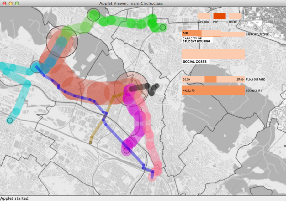
The application basically shows a map of Zurich, the travel routes to ETH Hönggerberg, and the traffic amount incurred by the students, as mapped on the routes (Kwan, 2000). The traffic and route representation is based on the sensing data previously obtained by case study using the methods of crowd-sourced mobile sensing. On the right side of the map is the simple user interface that can control the capacity of student housing, along with a bar graph to indicate the social costs.

Figure 10 and Figure 11 plot the out puts of two different scenarios. The user of the application also can further experiment with different student housing scenarios (i.e., locations and capacities of accommodation).

Figure 10.

Case A - Student housing evenly distributed over Zurich

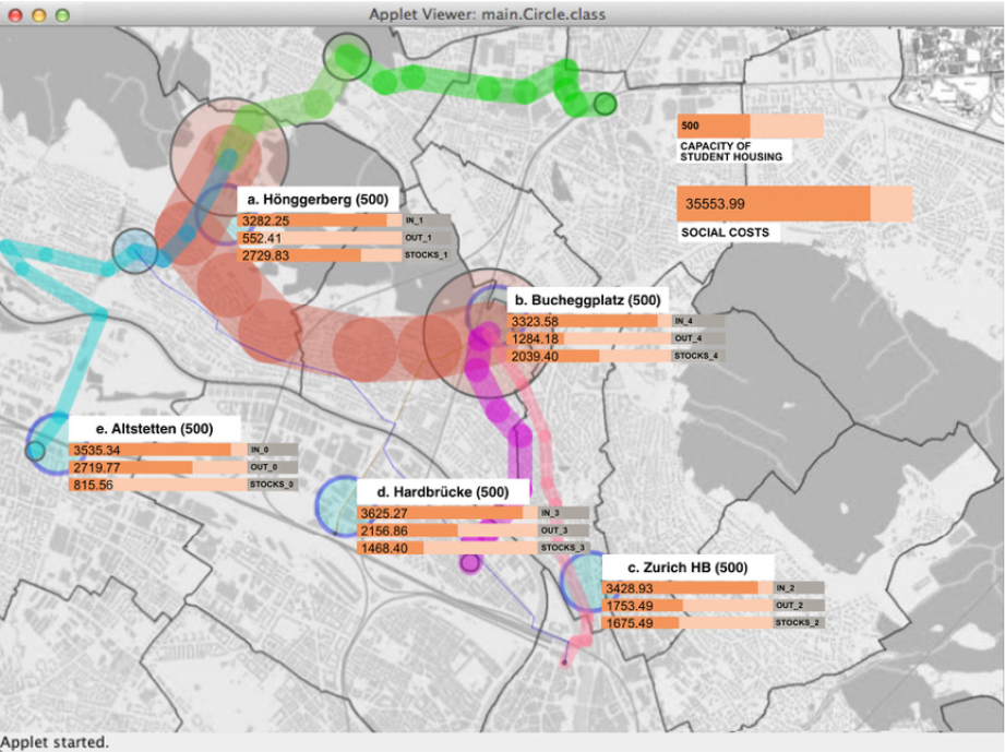
Figure 10 shows the results for five student housing projects built at locations in Zurich. The five different locations selected for the analysis were as follows: ETH Hönggerberg, Bucheggplatz, Zurich HB, Hardbrüke, and Altstetten. The other attribute, the scale of accommodations, was deemed to be 500 students.

- As could easily be expected, the analysis showed that constructing student housing in the Hönggerberg area provides a larger social costs savings than do the other places. And note that this result considers all stocks, flow-in, and flow-out values.

- The Altstetten area was determined to be the smallest social-cost-saving place. This was a reflection mainly of the flow-out value, 2719.77. The flow-out was indeed very high, whereas the flow-in, 3535.34, was similar to other places. More than 80% of the flow-in value was lost by the flowing-out.

- The flow-out value was defined on the basis of two major factors: distance from the campus, and distance from the other activity are as such as shopping and other cultural activities. Altstetten is not the farthest place from ETH Hönggerberg; nonetheless, it has the highest flow-out value. This means that it requires a relatively longer travel distance on average, or is associated with a relatively non-efficient travel mode compared with other places. In practice, the area has only one public travel mode to Hönggerberg, bus, which is the least efficient among the other public transportation modes; moreover, with respect to the distancefor non-commuting activities, the area is relatively farther than other places from, for example, the central area of Zurich, where most cultural activity occurs.

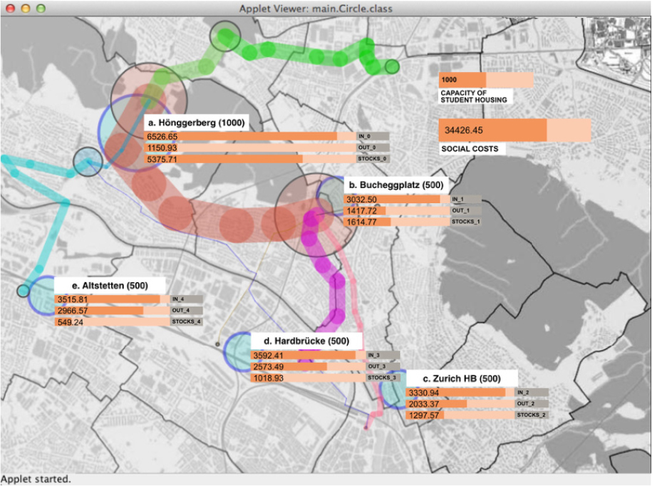
Figure 11 shows, as a sample result, how acapacity change of student housing brings about different effects in terms of social costs. For this simulation, the same basic conditions as in the previous setting were set, except for the capacity of student housing in the Hönggerberg area, which was increased from 500 students to 1000.

The following interesting results were obtained:

- The capacity doubles (500 to 1000) but the social costs savings (5375.71) is less than double (5459.66).

- By increasing the capacity of student housing, the savings amounts for other student housing are reduced.

- If the capacity of student housing increases, the total social costs also increase; however, the savings ratio per person decreases.

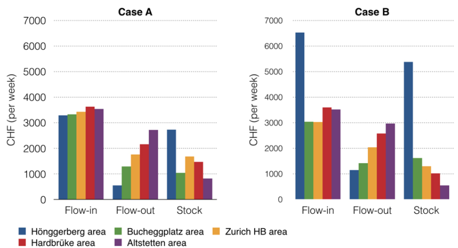
The following Figure 12 present the results of the analysis.

Figure 12 is a simple chart representation of the results in Figure 10 and Figure 11. Case A shows that the Hönggerberg area has a level of flow-in value similar to those of the other areas (since it is supposed to be on the same scale of building), but it also has a significantly low flow-out value. Therefore, eventually, the social costs savings amount, the “stock,” is the largest.

Figure 11.

Case B - Student housing highly concentrated at ETH Hönggerberg

Figure 12.

Social costs comparison between 'Case A’ and ‘Case B’ (CHF / week)

4. Discussion and Concluding

4.1 Understanding urban mobility: insights and limitations

This research's exploration of urban big data through the lens of social cost analysis provides a nuanced understanding of urban mobility. Our findings illustrate the significant impact of different transportation modes on the social and environmental fabric of urban areas. The variances in social costs observed across diverse student travel patterns emphasize the necessity of multi-modal transportation planning in urban development.

Yet, this study is not without its limitations. The reliance on mobile sensing data raises questions about the accuracy and representativeness of our findings. Future endeavors should aim to broaden data sources, including more in- depth environmental impact data, to solidify our conclusions. Additionally, applying these findings in various urban settings, beyond the confines of Zurich, could yield more comprehensive insights into urban dynamics.

For urban planners and policymakers, the practical implications of our research are clear. It offers a framework to better understand the social costs associated with different modes of transportation, guiding more sustainable and efficient urban planning decisions. This study underscores the importance of a balanced approach to urban development, one that weighs both the benefits and socio- environmental costs of urban activities.

4.2 Towards sustainable urban environments: a new perspective

In concluding, our research underscores the potential of mobile sensing data in shedding light on the social costs of urban travel behavior. The insights gained underscore how various transportation modes contribute to the overall social and environmental costs in urban settings. This study also highlights the critical role of participatory urban planning in fostering sustainable urban development.

The developed application serves as a practical tool, not only for visualizing but also for analyzing the social costs associated with different travel patterns. Such tools are crucial for urban planners and policymakers, enabling them to make more informed and sustainable decisions.

While our focus was on Zurich, the methodologies and insights garnered are applicable to other urban landscapes. This opens avenues for broader applications in urban planning and policymaking, emphasizing the integration of big data in urban planning. Our study represents a step forward in creating urban environments that are more livable, sustainable, and efficient for future generations.